

Spacecraft Engineering with Julia - Euler Angle Attitude Representation
Spacecraft Engineering with Julia - Euler Angle Attitude Representation
Using Euler angles to represent spacecraft attitude and model dynamics

Introduction
In my previous post, I modelled the attitude dynamics of a spacecraft using quaternion attitude representation. Since then, I figured out how to instead use Euler angles, which I find more intuitive. So, I’m writing a quick follow up to that article, this time numerically integrating the system of differential equations that use Euler angles instead of quaternions. The code for this article can be found at the following link: Spacecraft Attitude Control with Julia Part 1.5 - Euler Angle Attitude Representation.ipynb
Euler Angles
An important fact to remember is that the rates at which the Euler angles change is not equal to the components of a spacecraft’s angular velocity, i.e.,
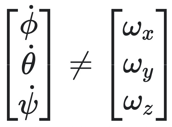
Where ϕ is the roll/rotation about the x axis, θ is the pitch/rotation about the y axis, and ψ is the yaw/rotation about the z axis.
I ran into this problem when I assumed that this is actually true (which this is valid if you are assuming small angles and rates). Instead, the relation between the Euler angle rates and spacecraft angular velocity are related by the following equation (for a 3-2-1 Euler angle rotation sequence) [1]:

Expanding these equations gives:
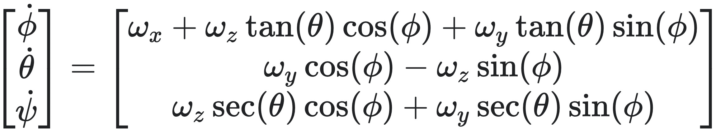
See the following link for a more in-depth derivation of the attitude kinematics of a 3-2-1 Euler angle sequence: Euler Angle Velocity of 321 Sequence
Implementation
With these equations, we can now rewrite the diffeq_euler function to instead use Euler angles to represent the spacecraft’s attitude. I covered the logic behind this function in greater depth in my last article, so if you want a better explanation of what’s going on, I recommend you reading that first. Like the previous quaternion implementation, we are using state-space representation, with the following state variable:

Using the equations for the derivative of the state variable, the diffeq_euler function can now be defined as:
function diffeq_euler(initial_conditions, time_span, params; solver_args...)
    function _differential_system(u, p, t)
        ϕ, θ, ψ, ω_x, ω_y, ω_z = u
        J_x, J_y, J_z, M_x, M_y, M_z = p

        return SA[
            ω_x + ω_z * tan(θ)*cos(ϕ) + ω_y*tan(θ)*sin(ϕ),
            ω_y*cos(ϕ) - ω_z*sin(ϕ),
            ω_z*sec(θ)*cos(ϕ) + ω_y*sec(θ)*sin(ϕ),
            (M_x(u, p, t) + (J_y - J_z) * ω_y * ω_z) / J_x,
            (M_y(u, p, t) + (J_z - J_x) * ω_x * ω_z) / J_y,
            (M_z(u, p, t) + (J_x - J_y) * ω_x * ω_y) / J_z
        ]
    end

    problem = ODEProblem(_differential_system, initial_conditions, time_span, params)
    solution = solve(problem; solver_args...)

    return solution
end
Using this function is exactly the same as the previous, except we now have a different state variable to use. Using the same parameters from the previous article, we get the following result:
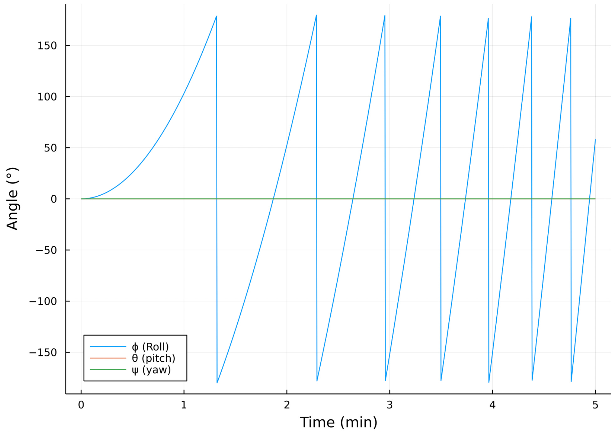
As can be seen, this is pretty much the exact same result as the previous article, so I’m happy that they both seem to be correct.
Conclusion
Using Euler angle representation, we have again successfully modelled the attitude dynamics of a spacecraft. Euler angles are a very intuitive method of representing the attitude of spacecraft, as well has not having any special constraints to impose, however they do have problems associated with them when using them for modelling. Specifically, Euler angle representations are hard to compose (see the link above), they have singularities, and each rotation sequence requires its own unique set of equations.
Now that I’ve covered actually modelling the dynamics of a spacecraft in this and the previous article, I will be focusing on implementing actual control of a spacecraft’s attitude in my next post. I’m really excited as I want to go into the GNC (guidance, navigation, and control) so working on this stuff is really interesting to me. I hope you learned something, and I’m looking forward to writing about more interesting stuff.
References
[1] A.H.J de Ruiter, C.J Danaren and J.R. Forbes, Spacecraft Dynamics and Control, John Wiley & Sons, 2013