

Spacecraft Engineering with Julia - PD Control
Spacecraft Engineering with Julia - PD Control
Actually implementing control this time!

Introduction
Now that we have a method to simulate the dynamics of a spacecraft's attitude (see the past two articles in this series), we can begin to implement control laws to make a spacecraft move the way we want. As always, I will not be delving into the nitty-gritty details and derivations of everything I talk about so feel free to research concepts yourself! You’ll learn a lot from people who are much smarter than me, I mainly like to focus on applying things and making visualizations.
The full code can be found at: Spacecraft Attitude Control with Julia Part 2 - PD Control.ipynb
PD Control
PD control is convenient because it works well in the time domain, where our simulations thus far have been within (I'll probably explore frequency domain modelling using ControlSystems.jl at a later point). As you'll soon see, it is pretty simple to implement with our diffeq_euler function.
For a PD controller the output torque is defined as:

Where θ is a Euler angle, Kp is the proportional gain, and Kd is the derivative gain. The ref subscript denotes a setpoint, or the target that the controller is trying to reach. From this equation it's clear as to why this is called a proportional-derivative controller, it is based on the control variable and its derivative.
Calculating the controller gains is not an exact science, typically estimates can be calculated and it's up to the engineer to tune the controller until it achieves satisfactory performance. I remember many labs during undergrad that consisted of waiting for our controllers to finish testing and adjusting their gains for hours on end. A good starting point for PD control is choosing a natural frequency ωₙ and damping ratio ζ. With these two values, the gains can be defined as:

Again, choosing these values for natural frequency and damping is not an exact science, however thinking in terms of natural frequency and damping gives a better intuition on how the system will behave. The plots below show different step responses of PD controllers with varying natural frequency and damping ratio values:


These graphs were made using ControlSystems.jl, a package that provides a large amount of controls-based functionality that is very similar to MATLAB. Also note that the plant used for these plots is the linearized version of Euler’s equation.
Implementing PD Control
To implement and test a PD controller, I’ll use a hypothetical scenario. Given a spacecraft with the following inertia matrix and starting attitude we’ll design a controller that settles at zero deviation with zero Euler angle rates within 1 minute:
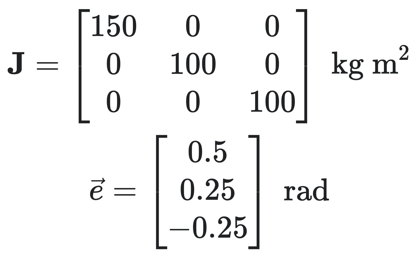
From this, we can define our vector of moments of inertia and setpoints:
Js = [150.0, 100.0, 100.0]
e_f = [0.0, 0.0, 0.0]
ė_f = [0.0, 0.0, 0.0]
Next, for the controller gains a natural frequency of 0.2 rad/s and damping ratio of 0.8 provide reasonable performance. The controller gains can be defined as a vector of values (one set of gains for each of the 3 principal axes):
ωₙ = 0.2
ζ = 0.8

Kp = Js .* ωₙ^2
Kd = 2 .* Js .* ωₙ .* ζ
Since the diffeq_euler function was written to accept any arbitrary function to calculate the torque, all we need to do is define the torque functions for a PD controller. Using the equation above the PD controller for the spacecraft’s roll can be defined as:
function Mx_func(u, p, t)
    ϕ, θ, ψ, ω_x, ω_y, ω_z = u
    ϕ̇ = ω_x + ω_z * tan(θ)*cos(ϕ) + ω_y*tan(θ)*sin(ϕ)

    return Kp[1]*(e_f[1] - ϕ) + Kd[1]*(ė_f[1] - ϕ̇)
end
The functions for the spacecraft’s pitch and yaw are also defined. The equations for the Euler angle rates can be found in my previous article.
With this minimal set up we can define the initial conditions, time span, and parameters to be inputted to the diffeq_euler function, and compute the solution:
tspan = [0.0, 60.0]
init = SA[0.5, 0.25, -0.5, 0.0, 0.0, 0.0]
params = [Js[1], Js[2], Js[3], Mx_func, My_func, Mz_func]

sol = diffeq_euler(init, tspan, params)
Since we are using Euler angle representation, we do not need to convert the resulting values, and we can directly plot them:
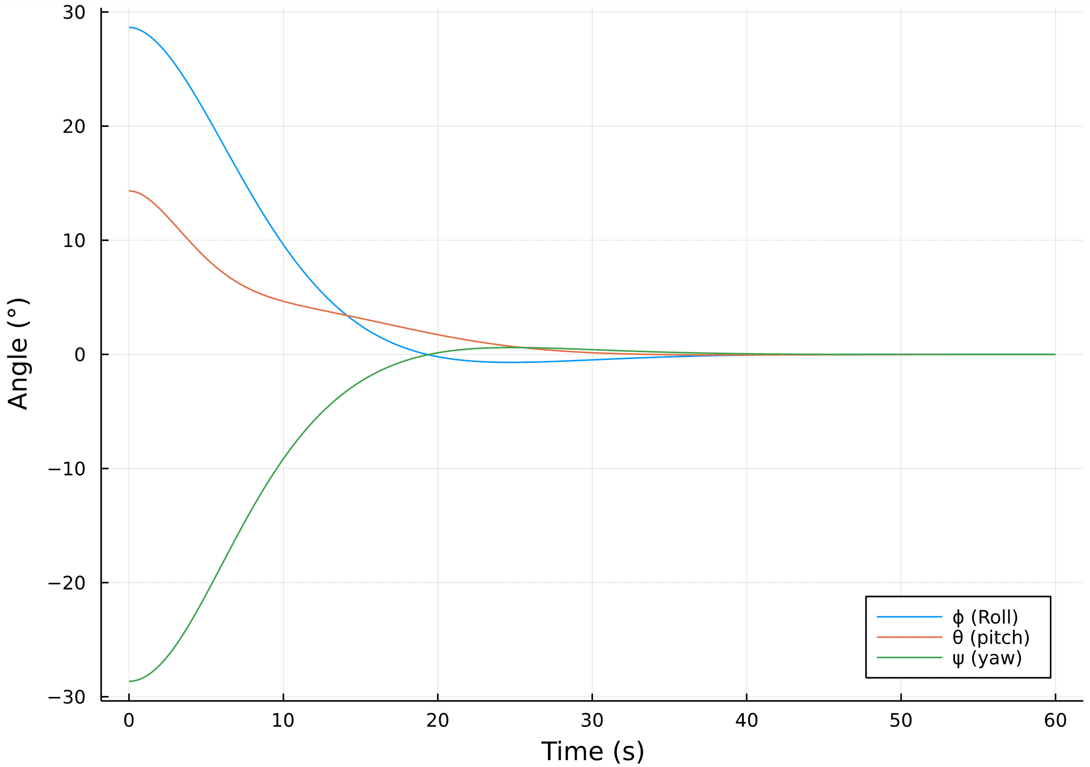
As can be seen, the controller managed to successfully maneuver the spacecraft from its starting position to pointing straight ahead without any deviation in any axis. Note that the system behaves slightly differently compared to the PD controller step responses above. This is due to the system of differential equations in this case being nonlinear, whereas the plots to showcase the effects of varying natural frequency and damping were created using the linearized version of Euler’s equation.
Extension: Modelling Uncertainty and Monte Carlo Simulations
A simple fact of life is that everything to an extent is uncertain. When designing a controller we may have clearly defined requirements but we always need to account for real-world uncertainties, one method of which is by using margins of safety. We can also test our controller in a variety of different scenarios, and a Julia package that really helps out in this aspect is the MonteCarloMeasurements.jl package.
Essentially this package models variables as distributions instead of fixed values. This allows us to propagate uncertainty throughout calculations, and as it turns out, simulations as well. This package works incredibly well with DifferentialEquations.jl, and this interoperability between packages is one of the main reasons why I love working with Julia. All you need to do is define variables with uncertainty and everything just works. I love it.
With this package, any variable can have uncertainty. What if our spacecraft has a range of possible moments of inertia? What if its angular velocity following separation is uncertain? These and many other scenarios can explored using this package. The plots from these calculations are also very nice to look at as well which is a big plus in my view.
For a simple example let’s take the same scenario we outlined above and change it a bit. Let’s just focus on the roll (x) axis for now. Let’s say we are modelling the attitude dynamics of a spacecraft after it is deployed from a launcher. We can introduce uncertainty by saying that the initial roll of the spacecraft will be 0.5 ± 0.05 rad, and the rate of roll will be ± 0.01 rad/s. Using MonteCarloMeasurements.jl, we can rewrite the init variable and implement the above measurements:
init_mcs = SA[
    0.5 + 0.05 * StaticParticles(100),
    0.0,
    0.0,
    0.01 * StaticParticles(100),
    0.0,
    0.0
]
This is the only modification that needs to be made, everything else remains the same. In this case, we are using 100 separate particles/samples to model the distribution of each variable.
Using the mcplot function, we can plot the trajectory of every single Monte Carlo simulation that was computed:
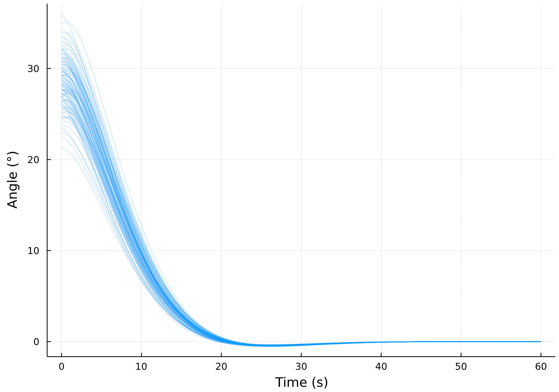
As can be seen, despite the range of different starting conditions the controller still manages to point the spacecraft towards zero deviation within 1 minute. Using the default plot function we can also create a ribbon plot that also shows the mean trajectory:

With these results we can see that the PD controller we selected still performs the required maneuver within 1 minute even with some varying roll and roll rate values.
Conclusion
Using PD control we have successfully implemented the control of a spacecraft’s attitude dynamics in Julia, as well as tested its robustness using uncertainty. Using MonteCarloMeasurements.jl opens up a new world of analyses that can be quickly implemented. I believe this package is incredibly powerful and useful for engineering, and I hope that more people begin considering Julia and its ecosystem for this type of work. But don't just take it from me, engineers at NASA have already implemented this kind of workflow in their tooling.
In the next article of this series we return to quaternions, and how to implement Quaternion Feedback control. If you want to see more of my work read some other articles I’ve written, also check out my website and Twitter. Thanks for reading!