Supersonic Inlet Design Using JuMP and Julia

Introduction

I know, this is a super niche application, but I think it's an interesting one regardless. My aim with this post is to both explain a bit of supersonic gas dynamics and provide a really basic introduction to using Julia and JuMP to solve a somewhat real-world aerospace engineering problem.

Earlier during my last semester of studying undergrad aerospace engineering, I had a project for my propulsion course that involved designing an inlet for use on a supersonic ramjet engine (among other things). The project required to come up with an optimal inlet at a specified number of oblique shockwaves and flight Mach number, and upon hearing this I knew I wanted to use Julia and JuMP to accomplish this task.

A bit of Gas Dynamics

Before I get too ahead of myself, I should explain what an oblique shockwave even is. I'm sure most people have a vague idea of what a shockwave is, but what does oblique shockwave mean?

So first off, shockwaves are regions of air that form within supersonic flow (i.e., flow moving faster than the speed of sound). A shockwave is a kind of disturbance or wall that causes supersonic flow to slow down to subsonic speeds upon crossing it. This explanation is super simple and not a very rigorous (one that would make my gas dynamics professor feel even more disappointed in me) but I think it gets the point across.

However, this description is specifically describing normal shockwaves, shockwaves that are normal (or perpendicular) to the direction of flow. Oblique shockwaves are similar to normal shockwaves, in that they are supersonic waves and slow down flow, but are also kind of different. Oblique shockwaves occur at some angle β from the direction of flow, called the shock angle. Oblique shockwaves do not actually make the flow of air slow down to subsonic speeds (not always, anyway), and oblique shockwaves actually change the direction of the flow. The angle of the flow past the shockwave is called the deflection angle, denoted θ.

So, when talking about shockwaves, normal shockwaves cause air to slow down from supersonic speeds, and oblique shockwaves cause air to change directions at supersonic speeds.

So what do shockwaves have to do with inlets for supersonic air-breathing engines? Without going into too much into the theory of these type of engines, they require air to be compressed in order to function decently well. Regardless of the type of shockwave, when flow goes through it, it slows down. So what happens when a bunch of air moving incredibly fast slows down? It compresses. All air-breathing engines require the intake air to be compressed, but a type of engine called ramjet engines are used specifically at supersonic speeds, which makes them a perfect candidate for using shocks to compress air, without needing mechanical compressors like the ones used on other types of aircraft gas turbine engines.

A schematic of a ramjet engine is shown below:

Source: NASA

Coding

With that short introduction out of the way, time to actually start coding. A while ago, some people way smarter than me figured out that there is always an optimal configuration of deflection and shock angles that result in the maximum amount of compression, or total pressure recovery, at a specific flight Mach number. This value occurs when the strength of each oblique shock in a supersonic inlet is equal to one another, i.e.:

This condition is useful as it gave me a check to ensure that the optimization worked and actually gave me the correct value.

So, this problem is perfect for some numerical optimization, as there is no analytical solution to this problem. Earlier on last year in 2021 I stumbled on the beautiful Julia programming language, and its various packages including JuMP. JuMP is a package that provides a universal interface for various mathematical optimizers. More specifically, it brings a domain-specific language to Julia for optimization. When my professor was explaining the project, I knew I wanted to solve this problem using JuMP, and I quickly set out to do so.

I quickly learned that throwing constraints and expressions at JuMP and hoping for the best was not a good strategy. My first few attempts to find the optimal solution ended in spectacular failures. I had to learn the hard way that optimization is not an easy task. I was never taught any kind of numerical optimization past simple implementations of Newton's method and the like, so I was mainly flying blind on what to do. I really did not have much experience with this before so I had to learn through trial-and-error quite a bit.

However eventually I finally came up with an optimization scheme that works for this specific problem, though of course the lessons I learned and ideas I came up with can be used for future projects.

To start, the required packages are loaded and the model is initialized. This is a non-linear optimization problem, so that’s why I went with Ipopt, a non-linear solver.

using JuMP, Ipopt
model = Model(Ipopt.Optimizer)

Next, some functions that describe gas dynamics equations need to be registered for use in the optimization. These equations are:

As can be seen, gas dynamics equations are very annoying to implement in programs. I’ll leave the code for these equations as an exercise for the reader. These equations are registered in the model with:

register(model, :post_oblique_mach, 2, post_oblique_mach, autodiff=true)

register(model, :oblique_shock_deflection, 2, oblique_shock_deflection, autodiff=true)

register(model, :oblique_P0_ratio, 2, oblique_P0_ratio, autodiff=true)

Next, defining control variables. In optimization, control variables are the variables an optimizer tunes in order to arrive at an optimal solution. In this case, I settled on using the shockwave angles, β. I initially wanted to set the deflection angles θ as my control variables, however this presented some problems that would take a little long to explain at depth. Basically, there is no direct method of calculating the shockwave angles with the limited information supplied, resulting in the optimizer to never arriving at a solution whenever I tried to implement this. So instead, shockwave angles. To specify the control variables:

@variables(model, begin
    β1 >= 0.2
    β2 >= 0.2
    β3 >= 0.2
end)

As seen, I also specified some initial starting angles, I basically did some trial-and-error of values until the solver actually reached a solution.

Next up, defining some expressions to use for optimization. The expressions in this case are just the other variables in the problem, the Mach numbers, deflection angles, and stagnation pressure ratios, but this time they are not independent control variables, they are values dependent on the shockwave angle:

@NLexpressions(model, begin
    # first shock
    θ1, oblique_shock_deflection(M1, β1)
    π1, oblique_P0_ratio(M1, β1)
        
    # second shock
    M2, post_oblique_mach(M1, β1)
    θ2, oblique_shock_deflection(M2, β2)
    π2, oblique_P0_ratio(M2, β2)

    # last shock
    M3, post_oblique_mach(M2, β2)
    θ3, oblique_shock_deflection(M3, β3)
    π3, oblique_P0_ratio(M3, β3)
end);

Next, specifying the constraints for this problem. These constraints are pretty straightforward, the first ensures that the Mach number of the flow past the last oblique shockwave is equal to the Mach number entering the final normal shock given in the problem, the next two make sure the variable Mach numbers are actually greater than 1, and that the deflection angles do not all equal up to 90 degrees, thereby generating an impassible wall:

@NLconstraints(model, begin
    post_oblique_mach(M3, β3) == Mn
    M2 >= 1
    M3 >= 1
    0 <= θ1 + θ2 + θ3 <= π/2
end);

Finally, we come to the objective of the optimization. As mentioned above, the goal of this optimization is to maximize the total pressure recovery, which is the product of all of the stagnation pressure ratios. Thus the objective definition is:

@NLobjective(model, Max, π1 * π2 * π3 * πn)

Where πn is the pressure ratio across the final normal shock, which is constant.

Now the model is set up and ready for optimization:

# optimization
set_silent(model)
optimize!(model)

# printing result
solution_summary(model, verbose=true)

And here is the output from the solver:

* Solver : Ipopt

* Status
  Termination status : LOCALLY_SOLVED
  Primal status      : FEASIBLE_POINT
  Dual status        : FEASIBLE_POINT
  Result count       : 1
  Has duals          : true
  Message from the solver:
  "Solve_Succeeded"

* Candidate solution
  Objective value      : 0.9339433812576963
  Primal solution :
    β1 : 0.5573768312905842
    β2 : 0.6695886799091497
    β3 : 0.8534322167406109
  Dual solution :

* Work counters
  Solve time (sec)   : 0.19000

As can be seen, the optimizer easily comes to a solution, at quite a fast time too (huge benefit of Julia if you don't know yet, once compiled this language is fast). As can be seen, at a flight Mach number of 2.4 we end up with a pressure recovery of 93.39%, a pretty good value I think. With these shock angles, all of the shock strengths end up being equal to around 1.2695085. Thus even though I did not even specify the optimal condition mentioned above, this code proves that that condition is correct, as all of the shock strengths are equal to each other at the optimal solution.

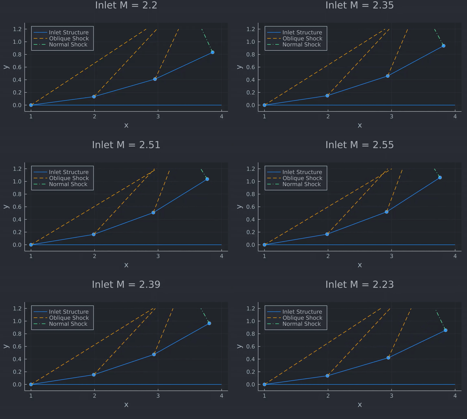
With the results found, the resulting geometry of the nozzle can be visualized:

Supersonic Inlet Geometry with 4 Shocks at Flight Mach of 2.4

As can be seen, this result is pretty similar to the example ramjet inlet shown above.

Extension - Variable Inlet Geometry

So, the optimal supersonic inlet layout is found for a flight Mach number of 2.4. However, at any other speed, this setup will no longer be optimal, thus it may be smart to design an inlet with variable geometry that moves during flight to ensure optimal compression at a range of speeds. Variable engine inlets exist in real life, like with the SR-71.

JuMP also works with vectors, allowing me to implement this variation of the original problem with minimal effort. Since the majority of the code is only slightly modified, here is the problem setup in its almost entirety:

n = 120
M1_vec = LinRange(2.2, 2.6, n)

var_model = Model(Ipopt.Optimizer)

register(var_model, :post_oblique_mach, 2, post_oblique_mach, autodiff=true)

register(var_model, :oblique_shock_deflection, 2, oblique_shock_deflection, autodiff=true)

register(var_model, :oblique_P0_ratio, 2, oblique_P0_ratio, autodiff=true)

# defining control variables
@variables(var_model, begin
    β1_vec[1:n] >= 0.47
    β2_vec[1:n] >= 0.47
    β3_vec[1:n] >= 0.47
end)

@NLexpressions(var_model, begin
    θ1_vec[j = 1:n], oblique_shock_deflection(M1_vec[j], β1_vec[j])
    π1_vec[j = 1:n], oblique_P0_ratio(M1_vec[j], β1_vec[j])

    M2_vec[j = 1:n], post_oblique_mach(M1_vec[j], β1_vec[j])
    θ2_vec[j = 1:n], oblique_shock_deflection(M2_vec[j], β2_vec[j])
    π2_vec[j = 1:n], oblique_P0_ratio(M2_vec[j], β2_vec[j])

    M3_vec[j = 1:n], post_oblique_mach(M2_vec[j], β2_vec[j])
    θ3_vec[j = 1:n], oblique_shock_deflection(M3_vec[j], β3_vec[j])
    π3_vec[j = 1:n], oblique_P0_ratio(M3_vec[j], β3_vec[j])
end);

# defining constraints
for i in 1:n
    @NLconstraints(var_model, begin
        post_oblique_mach(M3_vec[i], β3_vec[i]) == Mn
        M2_vec[i] >= 1
        M3_vec[i] >= 1
        0 <= θ1_vec[i] + θ2_vec[i] + θ3_vec[i] <= π/2
    end);
end

As can be seen, the control variables, expressions, and constraints must now be defined over a range, instead of at just a single point.

One caveat of using Ipopt is that using vectors in the objective definition is not allowed, thus a workaround is to maximize the sum of all total pressure recovery values:

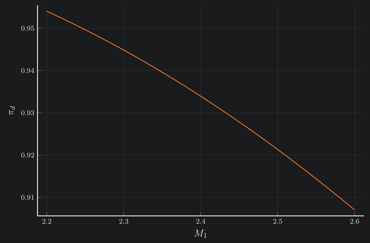
@NLobjective(var_model, Max, sum(π1_vec[i] * π2_vec[i] * π3_vec[i] * πn for i in 1:n))

With this set up, the model is ready to be solved. Now, the results come in ranges:

Optimal Shock and Deflection Angles over Range of Flight Mach Numbers

Total Pressure Recovery with Varying Flight Mach Number

I animated the changing shock and deflection angles over the range of flight Mach numbers, and posted the gif to my twitter:

Michal 🛰️ @astra_kawa

Supersonic inlet geometry and shock angles for optimal pressure recovery with three oblique shocks over a range of flight Mach numbers, made with Julia and JuMP + Ipopt

Wrapping Up

We come to the end of our little journey, using the amazing Julia programming language and JuMP packages to come up with an optimal inlet for a supersonic engine. I have not really done much optimization stuff in the past, but I found JuMP pretty easy to understand and use. From the code above, I'm sure you can also see how intuitive every single step is.