

Spacecraft Engineering with Julia - Using ModelingToolkit.jl
Spacecraft Engineering with Julia - Using ModelingToolkit.jl
Introducing an intuitive approach to modelling

Introduction
In the previous articles of this series, I introduced using Julia and the DifferentialEquations.jl package to model the attitude dynamics of spacecraft. I will now switch gears to using ModelingToolkit.jl for modelling instead, which provides a numerical-symbolic workflow, while still using DifferentialEquations.jl under the hood. To illustrate what this means, I will go through a simple example and then a more complex one.
Please read the previous Spacecraft Engineering with Julia articles to get an understanding of the math behind spacecraft attitude dynamics and control, as this article will just focus on using MTK.

Constant Torque About Single Axis
In this initial example of using MTK, I will recreate the example I covered in Spacecraft Engineering with Julia - Attitude Dynamics. In this example, we're modelling the attitude dynamics of a spacecraft being acted upon by a 0.1 Nm torque about the x axis.
First, the required packages we will be using are imported:
using ModelingToolkit, DifferentialEquations, PlotsNext, to start using MTK we first define the variables and parameters of the system:
@parameters t
D = Differential(t)

@variables ϕ(t) θ(t) ψ(t) ω_x(t) ω_y(t) ω_z(t)
@variables M_xs(t) M_ys(t) M_zs(t)

@parameters J_x J_y J_z
Using the parameters and variables macros we define the different values present in the system we are modelling. We consider parameters to be constant values and variables as dependent values, in this case dependent on time. Next, we use these parameters and variables to symbolically compose the equations of the system:
sys_simple = structural_simplify(ODESystem(
    [
        M_xs ~ 0.1,
        M_ys ~ 0.0,
        M_zs ~ 0.0,

        D(ϕ) ~ ω_x + ω_z * tan(θ)*cos(ϕ) + ω_y*tan(θ)*sin(ϕ),
        D(θ) ~ ω_y*cos(ϕ) - ω_z*sin(ϕ),
        D(ψ) ~ ω_z*sec(θ)*cos(ϕ) + ω_y*sec(θ)*sin(ϕ),

        D(ω_x) ~ (M_xs + (J_y - J_z) * ω_y * ω_z) / J_x,
        D(ω_y) ~ (M_ys + (J_z - J_x) * ω_x * ω_z) / J_y,
        D(ω_z) ~ (M_zs + (J_x - J_y) * ω_x * ω_y) / J_z,
    ],
    t,
    name = :spacecraft_model
))
The ~ operator is used to define the equations of the system. As can be seen, we no longer need to define functions for the torque values like we did in previous articles. We instead specify them directly in the definition of the system. The power and simplicity of this method will become a lot more evident in the next example.
Using the D variable we defined earlier, we can define the differential values of the system. Since this is an ODE system, each equation's left-hand side is the derivative of one of the system’s variables. Along with defining the equations of the system we also pass in the independent variable, in this case t. This is optional however I found that weird errors occur sometimes if you do not do this, so I just consider it best practice to add it in to make sure your program doesn't spit out some weird error. Finally we also specify the name of our system.
We also wrap the ODE system in a structural_simplify function, which as the name suggests, simplifies the system. It is quite powerful and I highly recommend reading the MTK docs to fully appreciate how much simplification this function can do. In this case, I call the function because we are modelling an ODE system, however in the system definition we can see that the torque equations are not differential equations. Thus the system is simplified by simply incorporating the torque values directly into the system.
With our system defined, we then define our initial conditions, parameters, and time-span variables:
u0_s = [
    ϕ => 0.0,
    θ => 0.0,
    ψ => 0.0,
    ω_x => 0.0,
    ω_y => 0.0,
    ω_z => 0.0,
]

p_s = [
    J_x => 100.0,
    J_y => 100.0,
    J_z => 100.0,
]

tspan_s = (0.0, 5*60.0)
We then define a DifferentialEquations.jl problem and pass it to the solve function along with a DE solver to get our solution:
prob_s = ODEProblem(sys_simple, u0_s, tspan_s, p_s, jac = true)
sol_s = solve(prob_s, Tsit5())
And that's it! I think this workflow is a lot easier and more intuitive than the one I have been using throughout the previous articles up until now. We can verify the solution by plotting the roll angle from the system:
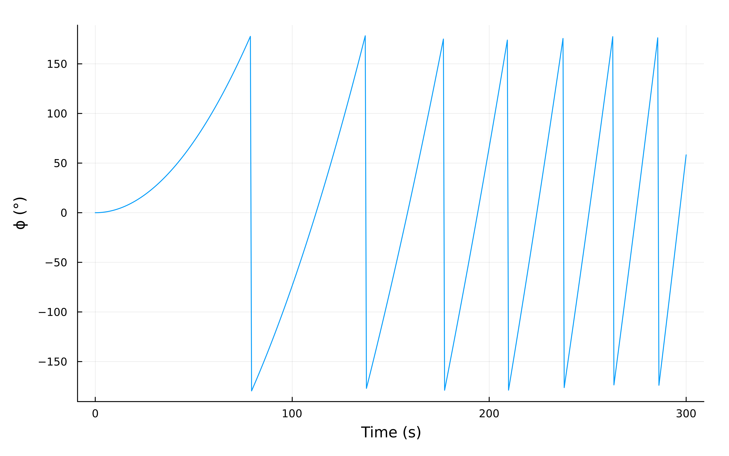
As can be seen, this is exactly the same result as we achieved in Spacecraft Engineering with Julia - Attitude Dynamics.
PD Controlled Spacecraft
Now for a more complex example. We will now implement the PD controlled spacecraft we modelled in the previous article in this series, Spacecraft Engineering with Julia - PD Control.
As before, we define the required variables and parameters for this system. We can utilize some of the previously defined ones, however this system requires its own specific variables and parameters. Specifically, we now have to define the desired Euler angles and derivatives of Euler angles for the controller, the controller gains, and the controller torque variables, which are now no longer simply functions of time:
@parameters ϕ_f θ_f ψ_f dϕ_f dθ_f dψ_f
@parameters Kp_x Kp_y Kp_z Kd_x Kd_y Kd_z

@variables M_x(Kp_x, Kd_x, ϕ_f, dϕ_f, ϕ)
@variables M_y(Kp_y, Kd_y, θ_f, dθ_f, θ)
@variables M_z(Kp_z, Kd_z, ψ_f, dψ_f, ψ)
With these variables and parameters, we can then define the system of equations:
sys_pd = structural_simplify(ODESystem(
    [
        M_x ~ Kp_x*(ϕ_f - ϕ) + Kd_x*(dϕ_f - D(ϕ)),
        M_y ~ Kp_y*(θ_f - θ) + Kd_y*(dθ_f - D(θ)),
        M_z ~ Kp_z*(ψ_f - ψ) + Kd_z*(dψ_f - D(ψ)),

        D(ϕ) ~ ω_x + ω_z * tan(θ)*cos(ϕ) + ω_y*tan(θ)*sin(ϕ),
        D(θ) ~ ω_y*cos(ϕ) - ω_z*sin(ϕ),
        D(ψ) ~ ω_z*sec(θ)*cos(ϕ) + ω_y*sec(θ)*sin(ϕ),

        D(ω_x) ~ (M_x + (J_y - J_z) * ω_y * ω_z) / J_x,
        D(ω_y) ~ (M_y + (J_z - J_x) * ω_x * ω_z) / J_y,
        D(ω_z) ~ (M_z + (J_x - J_y) * ω_x * ω_y) / J_z,
    ],
    t,
    name = :spacecraft_model_pd
))
Once again, we no longer have to write three separate functions for each torque in each direction, we can specify the torques directly in the system definition! You can probably start to understand how simple this workflow is compared to the one I used in the previous article. This code is a lot more intuitive and readable.
With the system defined, we again define the initial conditions, parameters, and time-span variables for the system:
u0_pd = [
    ϕ => 0.5,
    θ => 0.25,
    ψ => -0.5,
    ω_x => 0.0,
    ω_y => 0.0,
    ω_z => 0.0,
]

Js = [100.0, 100.0, 100.0]

ωₙ = 0.2
ζ = 0.8

Kp_val = Js .* ωₙ^2
Kd_val = 2 .* Js .* ωₙ .* ζ

p_pd = [
    J_x => Js[1],
    J_y => Js[2],
    J_z => Js[3],
    ϕ_f => 0.0,
    θ_f => 0.0,
    ψ_f => 0.0,
    dϕ_f => 0.0,
    dθ_f => 0.0,
    dψ_f => 0.0,
    Kp_x => Kp_val[1],
    Kp_y => Kp_val[2],
    Kp_z => Kp_val[3],
    Kd_x => Kd_val[1],
    Kd_y => Kd_val[2],
    Kd_z => Kd_val[3],
]

tspan_pd = (0.0, 60.0)
Next, we can define the ODE problem and plug it into the solve function to get our solution:
prob_pd = ODEProblem(sys_pd, u0_pd, tspan_pd, p_pd, jac = true)
sol_pd = solve(prob_pd, Tsit5())
We can now plot the spacecraft's Euler angles and angular velocity:
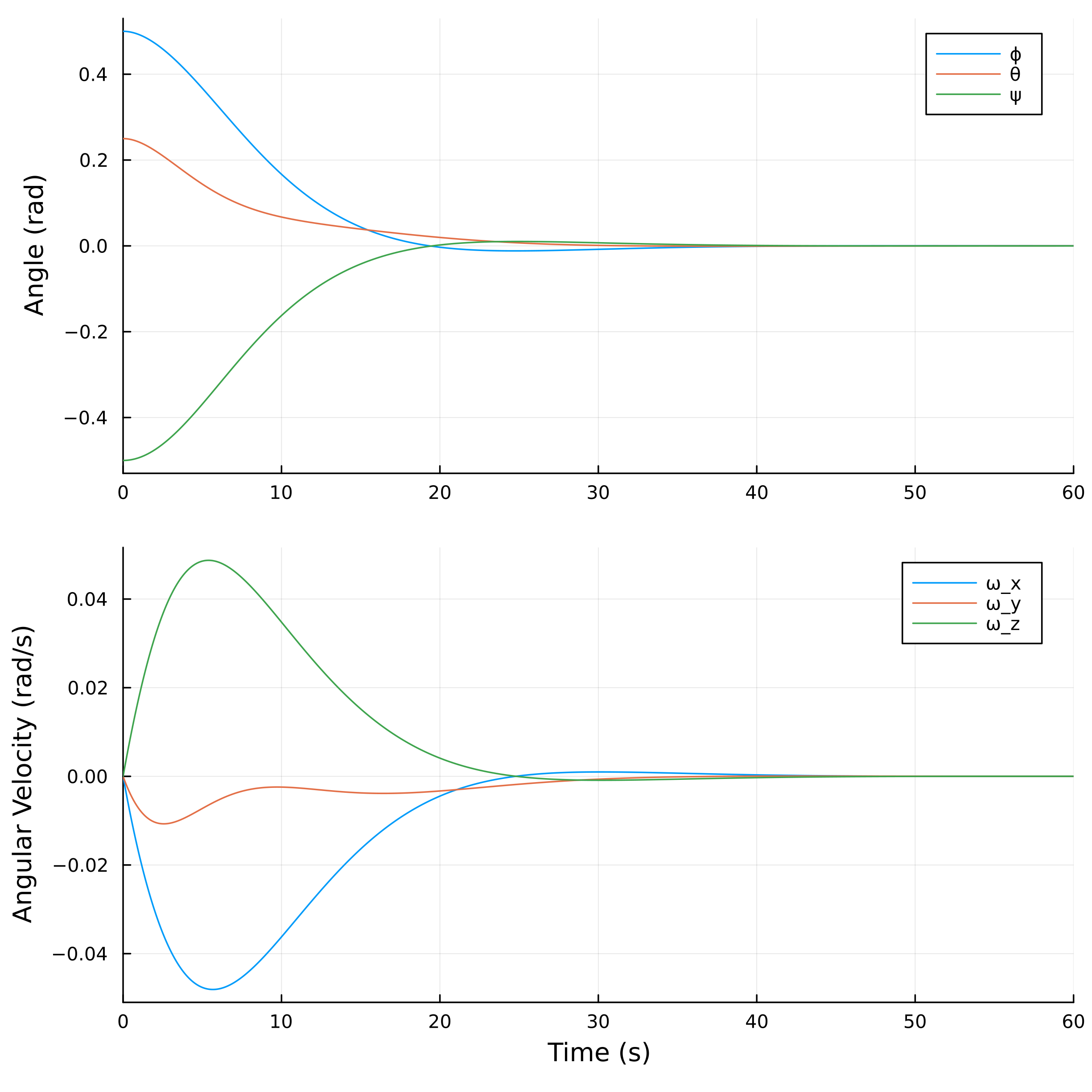
As can be seen, this is the same result we found in the previous article.
Conclusion
In conclusion, I hope I gave you a decent sense of the intuitive numerical-symbolic modelling workflow that ModelingToolkit.jl offers. I believe this workflow is a lot clearer compared to the one I have been using in the previous articles, and I will definitely be using it moving forward in future articles.
I have only scratched the surface of what you can do with ModelingToolkit.jl. The package has a lot to offer for engineering work, and I highly recommend reading through the docs and examples.
As always, the source code behind this and other articles can be found on my blog code GitHub repository. For more of my work and socials, please check out my website. If you’re interested in this kind of stuff, get into contact with me on Twitter or Mastadon! I’m always happy to talk and collaborate.